13.5 Solving Two General Equations in Two Variables

One nice feature of Newton's Method (and of Poor Man's Newton as well) is that it can easily be generalized to two or even three dimensions.

That is, suppose we have two standard functions, f and g of two variables, x and y. Each of the equations, f(x, y) = 0, and g(x, y) = 0 will typically be satisfied on curves, just as similar linear equations are satisfied on straight lines. And suppose we seek simultaneous solutions to both equations, which will then be at the intersections, if any, of these curves.

If we could solve either of the equations for x say, in terms of y, we could find a parametric representations of the curve solutions to it (with y as parameter), and use the divide and conquer method of the last section on the other function, cutting the parameter interval in half at each step as in one dimension.

This is a slow and steady method that can be implemented fairly easily. But it assumes we can obtain a parametric representation of one or the other curve.

We can always try Newton's method, which is fairly easy to implement in general.

To use Newton's method, we compute the gradients of f and g at some initial point, and find a new point at which the linear approximations to f and g defined by the gradients at the initial point are both 0. We then iterate this step.

To implement this method takes roughly three times the work of using Newton's method in one dimension. On the other hand three times almost nothing is still small.

This method suffers from the same problems as Newton's method suffers from in one dimension.

We may wander far from where we want to be in the xy plane, especially if we come to a point at which the gradients are small.

And of course two random curves need not intersect at all, so there may not even be a solution, or there could be many of them.

But again if we can start near a solution, under the right circumstances the method does very well indeed.

How do we set it up?

First you pick initial guesses of x₀ and y₀; on the spreadsheet, enter them in the first two columns (say). Then you need a column to enter f(x, y) and one for g(x, y); and one each for the x and y derivatives of f and g (four derivatives all together).

You now have all the information you need to compute x₁ and y₁. Once you have done this you need only copy everything down say 30 rows, and you can see what happens. If f and g go to zero, which means that x_i and y_i both converge, you will have a solution.

So how do we iterate?

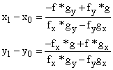
We must solve the two linear equations in x and y that state that the linear approximations to f and to g defined at (x₀, y₀) both are 0.

What are these equations? They are

And what are the solutions?

We can use Cramer's (ratio of determinant) rule to tell us that the solutions are

and

Of course all further iterations are identical to this one with the new guesses. Thus after entering these formulae once, copying them down is all that is necessary to apply the method.

Exercise 13.10 Try this method on a spreadsheet with the following function: f(x, y) = exp(x * y) - y² , g(x, y) = cos(x + y).
Find three solutions for which both variables are positive. How many such solutions are there?

The same approach can be implemented in three dimensions, though the amount of work required on a spreadsheet starts to be slightly tedious.

You have to enter three variables, three functions, their nine partial derivatives and of course Cramer's rule now involves the ratio of two three by three determinants each, now three times.

You could do it, though if you ever really wanted to, and actually find the solution to three arbitrary non-linear equations in three variables, with reasonable luck.